A steady drift in one direction that accumulates without limit, such as the rotation of the orbital plane. These dominate long-term prediction error.
EE 499 · Satellite Technologies
Week 4
Perturbations, TLEs & Time
Why a perfect two-body orbit drifts away from reality, and the time systems that turn an orbit into a ground track.
By the end: you should be able to explain what an orbit perturbation is and why propagation error grows, name the four dominant perturbations and where each matters, read the orbital fields of a TLE, describe how our ground-track visualizer turns a TLE into latitude and longitude, and follow the chain from UTC through Julian date and sidereal time to Earth rotation.
This week is conceptual. We do not derive perturbation equations and we do not implement a new propagator.
00 — HW2 help
Working through Homework 2
This section walks through Homework 2 the way you should approach it in an exam: identify what is given, choose the relation that connects the given to the unknown, and check the result against something you already know. The aim is that you can reproduce the reasoning, not that you can recall the final number.
00 — HW2 help
Question 1 — Geostationary orbit characteristics
Given / find: Find the classical orbital elements of a geostationary satellite, its apogee and perigee radii and heights, and its radial (angular) and linear speeds.
Approach: The three geostationary conditions from Week 3 — circular, equatorial, prograde — fix most of the elements immediately. Only the size has to be computed, and it follows from the period through Kepler's third law. Nothing here needs a look-angle formula.
00 — HW2 help
Geostationary orbit characteristics — working
- Circular orbit, so \(e\approx0\); equatorial orbit, so \(i=0^\circ\).
- Because \(e\approx0\) there is no distinction between apogee and perigee, so the right ascension of the ascending node \(\Omega\) and the argument of perigee \(\omega\) cannot be determined — a circular equatorial orbit has neither a unique node nor a unique perigee direction.
- Semi-major axis: \(a_{GSO}=42{,}164\ \text{km}\).
- With \(e=0\), \(r_a=r_p=a_{GSO}=42{,}164\ \text{km}\), so \(h_a=h_p=a_{GSO}-R_E\approx35{,}786\ \text{km}\).
- Radial (angular) speed: \(n=\dfrac{2\pi}{24\ \text{hr}}=0.2618\ \text{rad/hr}=7.2722\times10^{-5}\ \text{rad/s}\).
- Linear speed: \(v=n\,a_{GSO}=0.2618\times42{,}164=11{,}039\ \text{km/hr}\).
00 — HW2 help
Geostationary orbit characteristics — what goes wrong
00 — HW2 help
Question 2 — Antenna look directions to the Arabsat fleet
Given / find: For Riyadh, Cairo, Casablanca and New York, find the slant range, elevation and azimuth to satellites at \(20^\circ\text{E}\), \(26^\circ\text{E}\) and \(30.5^\circ\text{E}\).
Approach: Test visibility first. Computing look angles for a satellite that is below the horizon wastes time and produces a meaningless answer, so the visibility check is step one, not a check at the end.
00 — HW2 help
Antenna look directions to the Arabsat fleet — working
- Form the longitude difference \(|\phi_E-\phi_{SS}|\) and take the station latitude \(\lambda_E\).
- Read the maximum allowed separation \(|\phi_E-\phi_{SS}|_{\max}\) for that latitude from the visibility curves in the lecture notes.
- If \(|\phi_E-\phi_{SS}|<|\phi_E-\phi_{SS}|_{\max}\) the satellite is visible, so continue. Otherwise the satellite is not visible and you stop there.
- For every visible case compute \(\cos b\), then the slant range \(d\), then elevation and azimuth using the Week 3 relations.
00 — HW2 help
Antenna look directions to the Arabsat fleet — results
| Station | \(\lambda_E\) | \(\phi_E\) | \(\phi_{SS}=20^\circ\) | \(\phi_{SS}=26^\circ\) | \(\phi_{SS}=30.5^\circ\) |
|---|---|---|---|---|---|
| Riyadh | 25 | 45 | 37.11 · 49.61° · −132.19° | 36.85 · 53.86° · −140.83° | 36.70 · 56.56° · −148.54° |
| Cairo | 30 | 31 | 36.90 · 53.01° · −158.76° | 36.81 · 54.60° · −170.08° | 36.79 · 55.03° · −179.00° |
| Casablanca | 33.5 | −7.5 | 37.70 · 41.17° · 136.68° | 38.01 · 37.14° · 129.82° | 38.28 · 33.87° · 125.24° |
| New York | 40 | −74 | Not visible | Not visible | Not visible |
Each visible cell reads slant range \(d\ (\times1000\ \text{km})\) · elevation · azimuth.
00 — HW2 help
Antenna look directions to the Arabsat fleet — what goes wrong
00 — HW2 help
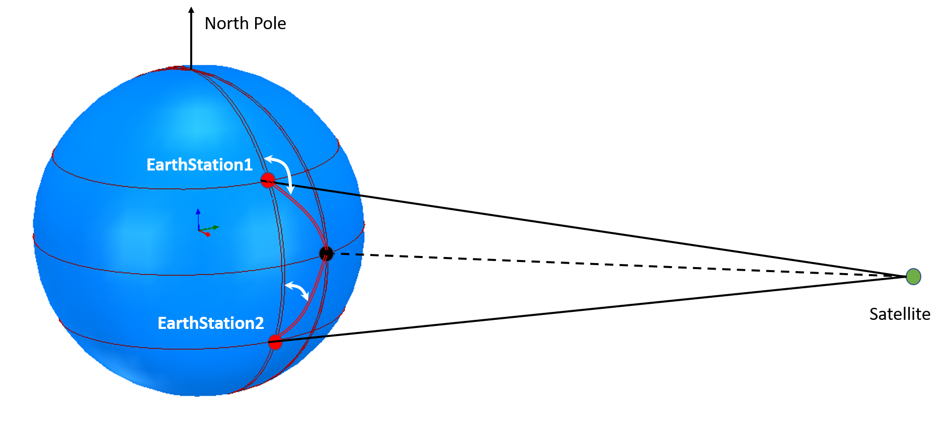
Question 3 — Two stations on one meridian (textbook Problem 3.4)
Given / find: One earth station at latitude \(30^\circ\text{S}\) and another at \(30^\circ\text{N}\) share the same longitude, and the satellite is \(20^\circ\) east of both. Find the look angles for each station and the round-trip time, counting propagation delay only.
Approach: Use the symmetry before reaching for the equations. The two stations are mirror images about the equatorial plane, so the geocentric angle \(b\), the slant range \(d\) and the elevation are identical for both. Only the azimuth differs, because one station looks north of east and the other looks south of east.
00 — HW2 help
Two stations on one meridian (textbook Problem 3.4) — the geometry
00 — HW2 help
Two stations on one meridian (textbook Problem 3.4) — working
- Both stations have \(|\phi_E-\phi_{SS}|=20^\circ\) and \(|\lambda_E|=30^\circ\), so both share the same \(b\), the same \(d=37{,}160\ \text{km}\) and the same elevation \(El=48.75^\circ\).
- The northern station points \(Az=143.95^\circ\); the southern station points \(Az=36.05^\circ\). The two azimuths sum to \(180^\circ\), which is the symmetry made visible.
- Round-trip time: \(\tau=\dfrac{2d}{c}\) with \(c=3\times10^{5}\ \text{km/s}\).
- \(\tau=\dfrac{2\times37{,}160}{300{,}000}=0.2477\ \text{s}=247.7\ \text{ms}\).
00 — HW2 help
Two stations on one meridian (textbook Problem 3.4) — what goes wrong
00 — HW2 help
Question 4 — Polar-mount antenna tilt
Given / find: Find the fixed angle of tilt for a polar-mount antenna at your home location, taken here as latitude \(\lambda_E=25^\circ\).
Approach: A polar mount rotates about one axis only, so its elevation is set once and then left alone. That fixed elevation \(El_0\) is the polar-mount relation from Week 3, not the general look-angle elevation formula.
00 — HW2 help
Polar-mount antenna tilt — working
- Slant range on the station's own meridian: \(d=\sqrt{R_E^{2}+a_{GSO}^{2}-2R_Ea_{GSO}\cos(25^\circ)}=36{,}489\ \text{km}\).
- Fixed elevation: \(El_0=\cos^{-1}\!\left(\dfrac{a_{GSO}}{d}\sin(25^\circ)\right)=60.7^\circ\).
00 — HW2 help
Polar-mount antenna tilt — what goes wrong
00 — HW2 help
Mistakes that cost marks — geometry and units
These are not specific to HW2. They are the recurring errors from Weeks 1 to 3, and they are worth checking before you submit anything.
| Radius versus altitude | Orbital radius is measured from Earth's centre, \(r=R_E+h\). Substituting an altitude into a formula that wants a radius is the single most common error. |
|---|---|
| Degrees versus radians | Trigonometric functions in MATLAB and in most languages take radians. Convert once, at the start, and stay in radians until you report. |
| Solar versus sidereal day | A geostationary orbit matches the sidereal day, \(86{,}164\ \text{s}\), not the \(86{,}400\ \text{s}\) solar day. |
00 — HW2 help
Mistakes that cost marks — constants and checks
| Units of \(\mu\) | \(\mu_E=398600.4418\ \text{km}^3/\text{s}^2\). If you work in metres you must use \(3.986\times10^{14}\ \text{m}^3/\text{s}^2\). Mixing the two silently produces answers wrong by \(10^{9}\). |
|---|---|
| Semi-major axis of an ellipse | \(a=(r_p+r_a)/2\) uses radii, not altitudes, and not the perigee radius alone. |
| Answer without a sanity check | Compare against something known: LEO periods are roughly 90 minutes, GEO is close to 24 hours, GEO altitude is near \(35{,}786\ \text{km}\). |
01 — Limits of the ideal model
Why a perfect orbit slowly stops being true
Everything in Weeks 1 to 3 rests on one idealisation: two point masses, one gravitational force, nothing else. Under that assumption the orbit is a fixed ellipse in inertial space, and the six classical elements are constants. Only the true anomaly \(\nu\) changes with time.
Real satellites do not behave that way for long. Earth is not a point mass and not a sphere, the atmosphere does not stop abruptly, and the Sun and Moon pull on the satellite as well. Each of these adds a small acceleration on top of the two-body term:
01 — Limits of the ideal model
One extra term changes everything
\[\ddot{\mathbf r}=-\frac{\mu}{r^3}\mathbf r+\mathbf a_{\text{perturbing}}\]
The perturbing acceleration is tiny compared with the main gravitational term — often smaller by a factor of \(10^{3}\) to \(10^{6}\). That is exactly why the two-body model is such a good first answer, and also why it is misleading: a small acceleration integrated over many orbits becomes a large position error.
01 — Limits of the ideal model
Small accelerations, integrated twice
This is why a prediction that is excellent for one orbit can be useless after a few weeks, and why tracking data must be refreshed. It is not that the mathematics of Weeks 1 to 3 is wrong; it is that the model those equations describe is incomplete.
02 — What is a perturbation
A small departure from the ideal problem
An orbit perturbation is any acceleration acting on the satellite that the two-body model does not include. The word is deliberate: these are not corrections to a mistake, they are physical effects that the idealised problem left out.
The useful consequence is that the six classical elements stop being constants. Instead of describing a fixed ellipse, they become slowly varying quantities — the orbit is still an ellipse at any instant, but that ellipse drifts, rotates and changes size over time. Engineers often describe perturbations by how the elements respond:
An oscillation that repeats each orbit or each day and averages out. These matter for precise pointing but not for long-term drift.
An effect that builds up when a perturbation period matches an orbital period, most familiar as east–west station-keeping in GEO.
03 — The four main perturbations
What pushes a satellite off the ideal ellipse
For this course the important distinction is the first one: secular effects are the reason an ideal propagation degrades with time, and the reason a TLE has an epoch attached to it.
Four effects account for nearly all of the departure from two-body motion for Earth satellites. Which one dominates depends almost entirely on altitude.
03 — The four main perturbations
What dominates in low orbits
Earth oblateness (\(J_2\))
Earth is not a sphere: it bulges at the equator by roughly \(21\ \text{km}\). The resulting non-spherical gravity field is described by a series of coefficients, of which \(J_2\approx1.083\times10^{-3}\) is by far the largest — about a thousand times bigger than every other term.
Its main effect is secular: the orbital plane rotates, so the right ascension of the ascending node \(\Omega\) drifts steadily, and the argument of perigee \(\omega\) rotates within the plane. This is the dominant perturbation for most orbits, and it is not always unwanted — Sun-synchronous orbits are designed so that the \(J_2\) drift of \(\Omega\) exactly matches Earth's motion around the Sun.
Atmospheric drag
The atmosphere thins gradually rather than ending, so satellites below roughly \(1000\ \text{km}\) fly through measurable air. Drag opposes the velocity and removes energy from the orbit.
Its signature is distinctive: because drag acts most strongly at perigee where the satellite is lowest and fastest, it lowers apogee first and gradually circularises the orbit, after which the whole orbit decays until re-entry. Drag depends on atmospheric density, which varies strongly with solar activity, and on the satellite's area-to-mass ratio. This is the effect that the \(B^{*}\) term in a TLE is there to capture.
03 — The four main perturbations
What dominates in high orbits
Sun and Moon gravity
The Sun and Moon attract the satellite as well as Earth. Because the perturbation grows with distance from Earth while Earth's own pull weakens, third-body effects are negligible in low orbits and significant in high ones.
For geostationary and highly elliptical orbits they are a leading effect, driving slow changes in inclination and node. Uncontrolled GEO satellites accumulate inclination at roughly \(0.8^\circ\) per year, which is why north–south station-keeping consumes most of a GEO satellite's fuel.
Solar radiation pressure
Sunlight carries momentum, so photons striking the satellite exert a small but continuous force. Unlike gravity it does not scale with mass, so it matters most for spacecraft with a large area-to-mass ratio — large solar arrays, or anything lightweight.
It is most important at high altitude where drag has vanished and the satellite spends most of its time in sunlight, and it is interrupted whenever the satellite passes through Earth's shadow.
04 — TLE refresher
Reading a two-line element set
A two-line element set is the standard published description of a satellite's orbit: two lines of exactly sixty-nine characters in a fixed-column format. It carries a set of mean orbital elements together with the time they describe and a drag term.
| Epoch | The instant the elements describe, written as a two-digit year and a fractional day of the year, in UTC. Every element in the set is valid at this moment; propagating away from it is where error accumulates. |
|---|---|
| Inclination \(i\) | Angle between the orbital and equatorial planes, in degrees. Same quantity as in Week 2. |
| RAAN \(\Omega\) | Right ascension of the ascending node: where the orbit crosses the equator going north, measured from the vernal equinox. |
| Eccentricity \(e\) | Orbit shape. Stored with an assumed leading decimal point, so the field 0006703 means \(e=0.0006703\). |
04 — TLE refresher
The remaining fields
| Argument of perigee \(\omega\) | Angle from the ascending node to perigee, measured in the orbital plane. |
|---|---|
| Mean anomaly \(M\) | Where the satellite is along the orbit at the epoch, expressed as the angle a fictitious uniformly-moving satellite would have. Convert to true anomaly through Kepler's equation, as in Week 1. |
| Mean motion \(n\) | Revolutions per day. This is how a TLE encodes orbit size: invert Kepler's third law to recover \(a\). |
| \(B^{*}\) drag term | A ballistic coefficient standing in for how strongly the atmosphere affects this satellite. It is not a classical orbital element — it exists purely so the propagator can model decay. |
A full field-by-field decoder, including the fixed-column layout and the parsing traps, is available in the TLE explainer lab.
04 — TLE refresher
Mean motion carries the orbit size
Mean motion gives the semi-major axis through the relation you already know:
\[n=\frac{2\pi}{T},\qquad a=\left(\frac{\mu_E}{n^{2}}\right)^{1/3}\]
05 — How our visualizer works
From orbital elements to an inertial position
The orbit and ground-track visualizer already in the course implements exactly the chain built up in Weeks 1 to 3. Nothing in it is hidden; it is worth knowing the stages because the same pipeline appears in every ground-track tool.
- Orbital elements. Start from \(a,e,i,\Omega,\omega\) and the mean anomaly at epoch — the same information a TLE carries.
- Two-body propagation. Advance the mean anomaly at the constant rate \(n\), then solve Kepler's equation \(M=E-e\sin E\) for the eccentric anomaly and convert to true anomaly. This is the step that assumes a perfect Keplerian orbit.
- Position in the inertial frame. Place the satellite in the perifocal frame, then rotate into ECI with \(R_z(\Omega)R_x(i)R_z(\omega)\). In ECI the orbit does not move.
05 — How our visualizer works
From an inertial position to a ground track
- Earth rotation. Rotate from ECI to the Earth-fixed frame by the Greenwich angle \(\theta_g\), which advances at one revolution per sidereal day, \(86{,}164.0905\ \text{s}\).
- Latitude and longitude. Convert the Earth-fixed position to a sub-satellite point, \(\phi=\arcsin(z/r)\) and \(\lambda=\operatorname{atan2}(y,x)\).
- Ground track. Plot successive sub-satellite points on the map. The familiar westward drift of each successive pass is Earth turning underneath a fixed inertial orbit.
SGP4 is the propagator that TLEs were actually designed for. Substituting it would change one stage of the pipeline and leave the rest intact.
05 — How our visualizer works
Where SGP4 would change this
| Today | Step 2 is ideal two-body motion. The elements are treated as constants and only \(M\) advances. |
|---|---|
| With SGP4 | Step 2 would include the perturbation effects that TLE mean elements assume — principally \(J_2\) and higher zonal harmonics, plus atmospheric drag through the \(B^{*}\) term. |
| Consequence | The predicted position would stay realistic much longer, because the secular drift of \(\Omega\) and \(\omega\) and the decay of the orbit would be modelled rather than ignored. |
| Unchanged | Steps 3 to 6. Once you have a position, the transformation to Earth-fixed coordinates, the sub-satellite point and the plotting are conceptually identical. |
We are not implementing SGP4 in this course and the visualizer is not being changed. The point is to know which single stage carries the modelling assumption, and what upgrading it would buy.
06 — UTC
One clock everybody agrees on
Coordinated Universal Time is the global civil time reference. It is generated from atomic clocks, and it is kept within a second of Earth's actual rotation by inserting occasional leap seconds. Local time zones are defined as offsets from it.
Satellite work needs a common time reference for an obvious reason: a position is meaningless without the instant it applies to. Ground stations on different continents must agree on when a pass begins, ranging measurements must be timestamped consistently, and orbit determination combines observations taken hours apart from different sites. All of it is done in UTC.
This is also how a TLE anchors itself. The epoch field is a UTC instant, written as a two-digit year followed by the day of the year including the fraction of a day. An epoch of 24145.51782528 means day 145 of 2024, at 0.51782528 of a day after midnight UTC — a little after 12:25 UTC.
07 — Julian date
Time as a single running number
Calendars are hostile to arithmetic. Months have different lengths, leap years interrupt the pattern, and subtracting two calendar dates requires special-case logic. Orbital mechanics needs to do arithmetic on time constantly — how many seconds since epoch, what is the interval between two observations — so it uses a continuous count instead.
The Julian date is that count: a single number giving the days, including the fraction of a day, elapsed since a fixed reference instant. Because it is just a number, the interval between two times is a subtraction, with no calendar logic at all.
In practice you convert the TLE epoch to a Julian date once, and every later question — how many seconds have elapsed, what is Earth's rotation angle now — becomes ordinary arithmetic.
07 — Julian date
A worked Julian date
Worked example. The standard reference epoch J2000.0 is 1 January 2000 at 12:00 UTC, which has Julian date
\[\text{JD}_{\text{J2000}}=2\,451\,545.0\]Ask for 1 January 2024 at 00:00 UTC. From 1 January 2000 to 1 January 2024 is 24 years containing 6 leap days (2000, 2004, 2008, 2012, 2016, 2020), so
\[24\times365+6=8766\ \text{days}\]That carries us to 1 January 2024 at 12:00 UTC. Midnight is half a day earlier, so
\[\text{JD}=2\,451\,545.0+8766-0.5=2\,460\,310.5\]The half-day offset is the usual source of error: a Julian day begins at noon, not at midnight. Some software avoids this with the Modified Julian Date, \(\text{MJD}=\text{JD}-2\,400\,000.5\), which does start at midnight.
08 — Sidereal time
Earth rotating beneath the orbit
Weeks 1 to 3 put the orbit in an inertial frame: ECI does not rotate, so the orbital plane stays fixed relative to the stars. A ground track, however, is drawn on a rotating Earth. Converting between the two viewpoints requires knowing how far Earth has turned, and that angle is what sidereal time measures.
The distinction matters because Earth's rotation relative to the stars is not the same as its rotation relative to the Sun. In one day Earth also moves along its orbit around the Sun, so it must turn slightly more than one full rotation for the Sun to return to the same meridian. The solar day is therefore about four minutes longer:
08 — Sidereal time
Two different days
\[T_{\text{sidereal}}=86{,}164.0905\ \text{s}\approx23^{\text{h}}56^{\text{m}}04^{\text{s}},\qquad T_{\text{solar}}=86{,}400\ \text{s}\]
08 — Sidereal time
The angle between the two frames
An orbit is fixed with respect to the stars, so it is the sidereal rate that governs how the Earth slides beneath it. The specific quantity needed is Greenwich Mean Sidereal Time — the angle \(\theta_g\) from the vernal equinox, which is the ECI \(x\)-axis, round to the Greenwich meridian, which is the Earth-fixed \(x\)-axis. Knowing \(\theta_g\) is exactly knowing the rotation between the two frames:
\[\theta_g(t)=\theta_g(t_0)+\omega_E\,(t-t_0),\qquad \omega_E=\frac{2\pi}{86{,}164.0905}\ \text{rad/s}\]
09 — The full chain
From a timestamp to a point on the map
The three time concepts are not separate topics. They are consecutive links in one chain that connects a clock reading to a ground track, and every satellite tracking tool walks it.
- UTC
- Julian date
- sidereal time
- Earth rotation angle
- ECI → Earth-fixed
- latitude & longitude
- ground track
Steps one to three are time-keeping, step four is a coordinate rotation, and steps five and six are geometry. The orbital mechanics of Weeks 1 to 3 supplies the inertial position that enters at step four.
09 — The full chain
Each link in the chain
| UTC → Julian date | Turn the calendar timestamp, including the TLE epoch, into one continuous number so intervals become subtraction. |
|---|---|
| Julian date → sidereal time | Use elapsed time to find the Greenwich mean sidereal angle \(\theta_g\) at the moment of interest. |
| Sidereal time → Earth rotation | \(\theta_g\) is the rotation between the inertial and Earth-fixed frames. |
| ECI → Earth-fixed | Rotate the propagated inertial position by \(-\theta_g\) about the polar axis. |
| Earth-fixed → latitude, longitude | \(\phi=\arcsin(z/r)\), \(\lambda=\operatorname{atan2}(y,x)\). |
| Points → ground track | Plot the sub-satellite points in sequence. |
10 — Check yourself
Reason across the week
1 · Perturbations
Which perturbation dominates for an uncontrolled satellite in a \(400\ \text{km}\) circular orbit?
10 — Check yourself
Reason across the week
2 · Time systems
Why is sidereal time, rather than solar time, used to find Earth's rotation angle for a ground track?
11 — Week summary
An ideal model, and what it leaves out
Perturbations
Small accelerations outside the two-body model. \(J_2\) and drag dominate low orbits; third-body gravity and radiation pressure dominate high ones.
TLE
Mean elements plus an epoch and a drag term, designed for a propagator that models perturbations.
Our visualizer
Two-body propagation into ECI, then Earth rotation, then a sub-satellite point. SGP4 would replace only the propagation stage.
Time
UTC gives a common instant, Julian date makes it arithmetic, sidereal time gives Earth's rotation angle.
EE 499 · Week 4
Week 4 complete
- HW2 review
- ideal-model limits
- perturbations
- TLE refresher
- ground track
- time systems
The two-body model is exact for a problem that does not quite exist. Real orbits feel Earth's equatorial bulge, the residual atmosphere, the Sun and Moon, and sunlight itself. These perturbations make the classical elements drift, which is why an ideal propagation degrades with time and why every TLE carries an epoch.